Correlation *is* causation!

- at least mathematically

We all know the old mantra drilled into us since the first week of Intro to Research Methods: “correlation is not causation”. This is, of course, true. But that won’t stop me from making a little stats sleight-of-hand to get you thinking more about what this means.

Too often, I see in manuscript critiques that reviewers rely on the analysis used to gain insights into the design and hypothesis without really considering that there are many ways to answer the same causal question. Here, I will illustrate a simple example of this.

I will show you that a Pearson’s correlation is identical to a Student’s t-test. The former is often attributed to studies looking at associations (non-causal), while the latter is attributed to experiments looking for effects (causal). But they are both identical (mathematically).

Here is some data to start us off:

# Set a seed to obtain identical results
set.seed(1410)

# Make two groups of n = 30 each
group <- rep(0:1, each = 30)

# Make a test score DV that varies a bit between groups (M1 = 50, M2 = 60)
score <- c(rnorm(30, 50, 10), rnorm(30, 60, 10))

Above, I envision a simple study looking at the difference in scores between two groups. This is a classic experimental setup. But this by itself doesn’t say much about the hypothesis or whether the study is an experiment, quasi-experiment, or purely observational. Maybe the assignment was random to the two groups (experiment), maybe group was assigned based on days of the week (quasi), or maybe it is just two groups from different countries (observational).

Given this design, I will of course use…Pearson’s correlation:

cor.test(group, score)

I now assume you are making this face:

Clearly, clearly, this is a design that begs for the t-test to be used. But, let’s see the results:

> cor.test(group, score)

	Pearson’s product-moment correlation

data:  group and score
t = 2.4766, df = 58, p-value = 0.0162
alternative hypothesis: true correlation is not equal to 0
95 percent confidence interval:
 0.06004559 0.52217469
sample estimates:
      cor 
0.3092551 

We find an r = 0.39, t = 2.48, and p = .0162. But, surely this is the wrong test for this design and data structure, so we don’t know what to make of it. We must use a t-test to find the true effect!

# Use var.equals = TRUE to get Student's t-test (default is Welch's)
t.test(score ~ group, var.equal = TRUE)

Now, we can see the true result:

> t.test(score ~ group, var.equal = TRUE)

	Two Sample t-test

data:  score by group
t = -2.4766, df = 58, p-value = 0.0162
alternative hypothesis: true difference in means between group 0 and group 1 is not equal to 0
95 percent confidence interval:
 -13.672398  -1.449888
sample estimates:
mean in group 0 mean in group 1 
       50.53325        58.09439 

Indeed, now we see that the result is…the same… t = 2.48, p = .0162

So what gives? Let’s look at the math here for a second. For two continuous variables X and Y, the Pearson correlation r tests whether there is a linear relationship between them. The formula for r is:

\(r = \frac{\sum (X_i - \bar{X})(Y_i - \bar{Y})}{\sqrt{\sum (X_i - \bar{X})^2 \sum (Y_i - \bar{Y})^2}}\)

The test statistic for the correlation is:

\(t = \frac{r\sqrt{n - 2}}{\sqrt{1 - r^2}}\)

This t-value follows a t-distribution with n−2 degrees of freedom. This is also just like a two-sample t-test!

If the correlation is between a continuous and a binary variable, the results will be identical. That is because the correlation between the binary variable and the continuous variable is mathematically equivalent to the point-biserial correlation, which is just a special case of Pearson’s r (r_pb).

And the test of whether that correlation differs from 0 is exactly the same as the independent-samples t-test testing whether the two group means differ.

Proof

Suppose X is not continuous, but binary: coded 0 for Group 1, and 1 for Group 2.
Let Y be a continuous outcome (test scores). Then we can write:

\(\bar{Y}_1 = \text{mean of } Y \text{ when } X = 1, \quad \bar{Y}_0 = \text{mean of } Y \text{ when } X = 0\)

The t-test for the difference in means is (n1 and n0​ are the group sizes):

\(t = \frac{\bar{Y}_1 - \bar{Y}_0}{s_p \sqrt{\frac{1}{n_1} + \frac{1}{n_0}}}\)

Now, let’s look at the correlation. When X is coded 0/1, the point-biserial correlation is (s_Y is the standard deviation of Y across all observations, and n=n1+n0):

\(r_{pb} = \frac{\bar{Y}_1 - \bar{Y}_0}{s_Y} \sqrt{\frac{n_1 n_0}{n^2}}\)

If you substitute this r_pb into the correlation test statistic:

\(t = \frac{r_{pb}\sqrt{n - 2}}{\sqrt{1 - r_{pb}^2}}\)

and you simplify, you get the exact same formula as the t-test above. Same t, same degrees of freedom, same p-value.

TL;DR testing whether the correlation differs from zero is identical to testing whether the group means differ. So in this case — correlation is causation (mathematically speaking).

Bonus: It’s all just linear models anyway

The unifying language

For completeness, we can express both tests as linear regression.

\(Y_i = \beta_0 + \beta_1 X_i + \varepsilon_i\)

For brevity, I show only the t-statistic formula of the linear model:

\(t = \frac{\hat{\beta}_1}{SE(\hat{\beta}_1)}\)

If we analyse the data using a simple linear model we get the exact same results:

summary(lm(score ~ group))

Check the output:

> summary(lm(score ~ group))

Call:
lm(formula = score ~ group)

Residuals:
    Min      1Q  Median      3Q     Max 
-33.655  -7.044   0.351   7.796  24.248 

Coefficients:
            Estimate Std. Error t value Pr(>|t|)    
(Intercept)   50.533      2.159  23.408   <2e-16 ***
group          7.561      3.053   2.477   0.0162 *  
---
Signif. codes:  0 ‘***’ 0.001 ‘**’ 0.01 ‘*’ 0.05 ‘.’ 0.1 ‘ ’ 1

Residual standard error: 11.82 on 58 degrees of freedom
Multiple R-squared:  0.09564,	Adjusted R-squared:  0.08005 
F-statistic: 6.134 on 1 and 58 DF,  p-value: 0.0162

Same p-value = .0162, df = 58, and t-statistics (F = t^2) = 2.476. This is because all classical inference in linear models (t, F, r) comes from the same foundation: least squares estimation. The t-test is not a “special case”; it’s just regression with a binary predictor. Correlation isn’t just about co-movement; it’s the geometry of linear prediction.

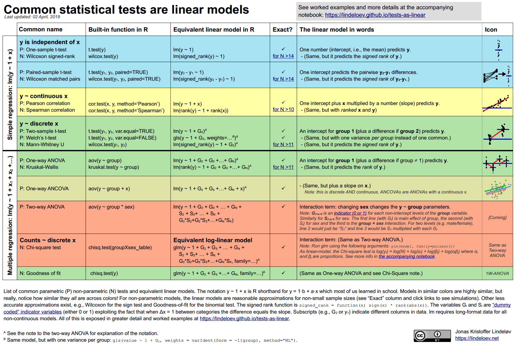
Jonas Kristoffer Lindelev made this very nice cheatsheet for common tests and their linear model syntax equivalent to demonstrate this fact. It is a useful read. That said, there are reasons why some of these special case tests were invented, so do not jump to conclusions about their equivalence (see this post by Stephen Senn about ANOVA that is quite insightful; it shows that we can “bypass” some test assumptions by designing our way around them).

Conclusion

Nothing in this post is new knowledge. But, it is the start of teaching term, and I often see educators (myself included) do something like “Today, we will learn about associations” and teach a correlation, then next week say “Today, we will learn about effects” and teach the t-test. This, I found, makes student believe the “causal” bit of “causal inference” is due to the test we use, not the hypothesis and design employed.

So next time someone says “correlation isn’t causation,” you can reply:

“Well, technically…if your correlation is with a dummy-coded variable, it kind of is.”

(Just don’t try that in a peer review rebuttal)

P.S. To make sure no one goes away with the wrong conclusion from my post. I am *not* actually saying that “correlation is causation”. I’m simply illustrating that the *model used* does not confer any magical causal properties to a study. Your study needs to be set up to make causal claims, you can’t save it post hoc.